Digital Signal Processing Concepts

In this blog post, I'll be diving into some concepts of digital signal processing (DSP). Most of them I had to learn before starting to work with models that take audio files as input and therefore, require some preprocessing steps.

The concepts I'll briefly discuss here are:
1. Fourier transforms
2. Sampling rate
3. Discrete Fourier Transform
4. Short Time Fourier Transform
5. Mel-spectrograms

Before digging into each of the topics, something cool to remember is how we humans perceive audio. In our ears, whenever we hear something, basically the air pressure variation (sound waves) makes some tiny bones inside our ear vibrate, this way our brain can identify each of the sounds such as barks, music, noise, and so on depending on some features they have.

1. Fourier Transforms

The main goal of a Fourier transform is to split the components (frequencies) that are forming an audio file. A very used image to illustrate how the Fourier Transform works is the Pink Floyd album cover:

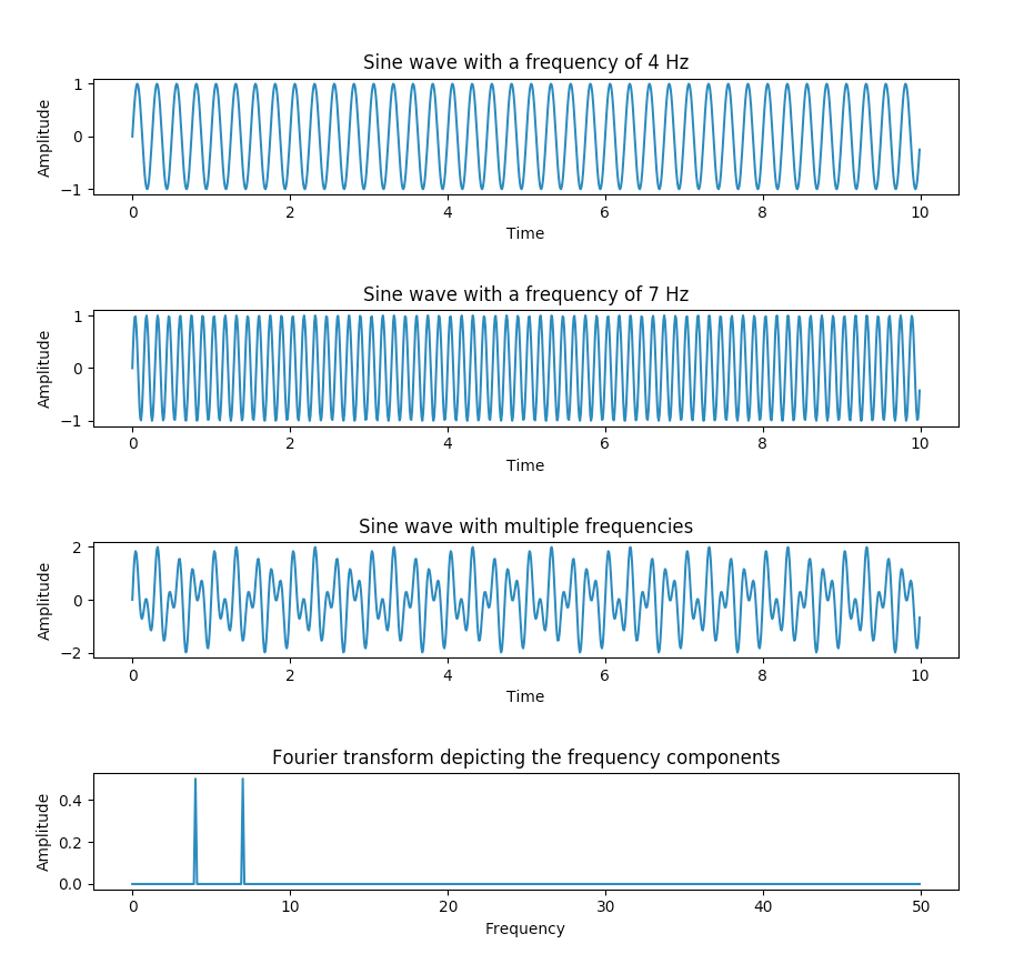
So if we input an audio file and apply a Fourier transform on it, we would end up having something like this:

Image from pythontic

The CFT (Continuous Fourier transform) formula is the following:

Where k is each of the frequencies we want to analyze and F is the function that produces the waveform.

Something worth mentioning is that we can also compute the IFT (Inverse Fourier Transform) - which takes as input the frequency and magnitude spectrum and converts it to the sound wave again (we lose the information about the phase though).

2. Sampling rate

Whenever we record something using a microphone, it gets the air pressure variations within a certain period. In nature, sound waves have an analogic format (It's continuous), but whenever we store these sound waves we need to take a bunch of samples of them, so we can store them properly in a discrete format. The process of taking these few "moments" of the audio it's called sampling. We see a lot of 44.1khz sample rates but we don't realize (At least for me until that point) what that really means. A 44.1Khz recorded audio means that for each second, we extracted 44100 samples - yeah that's a lot. Fortunately, there are methods that allow us to upsample (Increase the number of samples per second) or downsample (Reduce the number of samples per second).

3. Discrete Fourier Transform

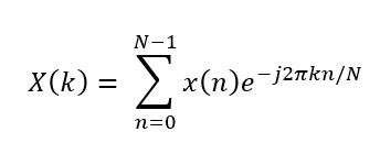
Now that we know that our audio files are stored in a discrete format, we can't use the Fourier transform formula anymore, since it was only applied to continuous signals. To overcome that, we can take the correspondent operation of the integrals in the discrete scenario (which is the summation). This way, we can formulate the DFT equation like this:

Note on fast transforms: The Fourier transform big-O notation is O(N2), and by taking some of the audio signals properties such as symmetries and periodicities using a divide-and-conquer approach, we can speed this computation up to O(N log N) with the Fast Fourier Transform to compute data more efficiently.

4. Short Time Fourier Transform

When I first started to study the Fourier transform something was always a little weird. How could we extract features from the whole audio and also keep track of the time each of that features happened?

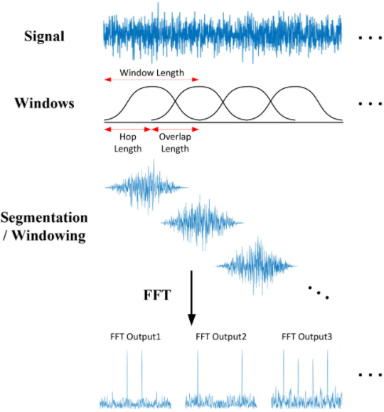
The answer for that came after understanding the short-time Fourier transform (STFT) which consists of applying FFT (Fast Fourier transforms) on little segments of the audio. This way we would know where each of the frequencies happened and also their magnitude.

A few parameters are required to be set up before computing such as:
hop size: Which defines how many samples to skip;
window size: On how many samples to apply the fast Fourier transform;
overlap length: The number of how many samples are going to be in overlap within two consecutive windows

stft image

5. Mel spectrograms

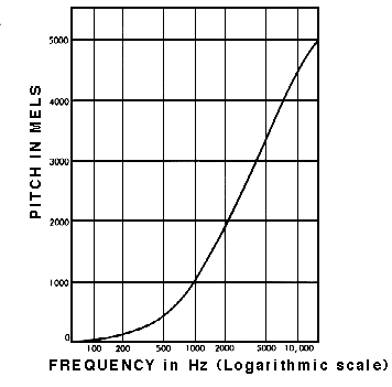
Cool, now that we have all the concepts shown above, what's missing to make my model perceive sounds as humans do? Basically, our species can't hear that well all frequencies in the spectrum, so the Mel scale is applied to a spectrogram to try to match what our ears can hear properly. This conversion isn't always needed but it's found out that converting spectrograms to the mel-scale helps models learn faster.

So now we have everything ready to extract features from our audio files and apply them to our CNN models or so! Hope you enjoyed :)

Share on: